本指南训练了一个神经网络模型,以对运动鞋和衬衫等服装图像进行分类。你可以不了解所有的细节,这是一个完整的TensorFlow程序的快速概述,详细内容会在你开始的时候解释。
本指南使用tf.keras,一个高级API来中构建和训练TensorFlow模型。
 1
 2
 3
 4
 5
 6
 7
 8
 9
10
11
12
13
|
from __future__ import absolute_import, division, print_function, unicode_literals

# TensorFlow and tf.keras
import tensorflow as tf
from tensorflow import keras

# Helper libraries
import numpy as np
import matplotlib.pyplot as plt

print(tf.__version__)

2.0.0
|
导入Fashion MNIST数据集
本指南使用Fashion MNIST数据集,其中包含10个类别的70,000个灰度图像。这些图像以低分辨率(28*28像素)显示衣服的各个物品,如下所示:
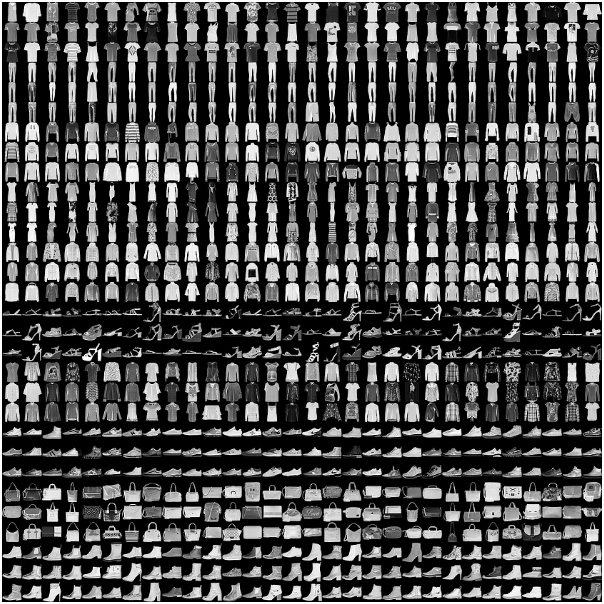
Fashion MNIST旨在替代经典MNIST数据集,该数据集通常被用作计算机视觉机器学习程序的“Hello, World”。MNIST数据集包含手写数字(0、1、2等)的图像,其格式与你将在此处使用的衣服的格式相同。
本指南将Fashion MNIST用于多种用途,因此它比常规MNIST更具挑战性。两个数据集都相对较小,用于验证算法是否按预期工作。它们是测试和调试代码的良好起点。
这里,使用60,000张图像来训练网络,使用10,000张图像来评估网络学习对图像进行分类的准确程度。你可以直接从TensorFlow访问Fashion MNIST。直接从TensorFlow导入和加载Fashion MNIST数据:
 1
 2
 3
 4
 5
 6
 7
 8
 9
10
11
|
fashion_mnist = keras.datasets.fashion_mnist
(train_images, train_labels), (test_images, test_labels) = fashion_mnist.load_data()

Downloading data from https://storage.googleapis.com/tensorflow/tf-keras-datasets/train-labels-idx1-ubyte.gz
32768/29515 [=================================] - 0s 0us/step
Downloading data from https://storage.googleapis.com/tensorflow/tf-keras-datasets/train-images-idx3-ubyte.gz
26427392/26421880 [==============================] - 0s 0us/step
Downloading data from https://storage.googleapis.com/tensorflow/tf-keras-datasets/t10k-labels-idx1-ubyte.gz
8192/5148 [===============================================] - 0s 0us/step
Downloading data from https://storage.googleapis.com/tensorflow/tf-keras-datasets/t10k-images-idx3-ubyte.gz
4423680/4422102 [==============================] - 0s 0us/step
|
加载数据集将返回四个NumPy数组:
train_images和train_labels数组是模型用来学习的数据训练集。- 针对测试集
test_images和test_labels数组对模型进行测试。
图像是28*28 NumPy数组,像素值从0到255不等。标签是一个整数数组,范围从0到9。这些对应于图像所代表的衣服类别:
| 标签 |
类 |
| 0 |
T-shirt/top |
| 1 |
Trouser |
| 2 |
Pullover |
| 3 |
Dress |
| 4 |
Coat |
| 5 |
Sandal |
| 6 |
Shirt |
| 7 |
Sneaker |
| 8 |
Bag |
| 9 |
Ankle boot |
每个图像都对应一个标签。由于类名不包含在数据集中,因此将它们存储在此处,以便后面在绘制图像时使用:
1
2
|
class_names = ['T-shirt/top', 'Trouser', 'Pullover', 'Dress', 'Coat',
               'Sandal', 'Shirt', 'Sneaker', 'Bag', 'Ankle boot']
|
研究数据
在训练模型之前,让我们先研究一下数据集的格式。下面显示训练集中有60,000张图像,每张图像表示为28*28像素:
1
2
|
train_images.shape
(60000, 28, 28)
|
同样,训练集中有60,000个标签:
1
2
|
len(train_labels)
60000
|
每个标签都是0到9之间的整数:
1
2
|
train_labels
array([9, 0, 0, ..., 3, 0, 5], dtype=uint8)
|
测试集中有10,000张图像。同样,每个图像都表示为28*28像素:
1
2
|
test_images.shape
(10000, 28, 28)
|
测试集包含10,000个图像标签:
1
2
|
len(test_labels)
10000
|
预处理数据
在训练网络之前,必须对数据进行预处理。如果你检查训练集中的第一张图像,将会看到像素值在0到255范围内:
1
2
3
4
5
|
plt.figure()
plt.imshow(train_images[0])
plt.colorbar()
plt.grid(False)
plt.show()
|
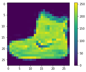
在将这些值输入神经网络模型之前,将它们缩放到0到1的范围。为此,将这些值除以255。以相同的方式预处理训练集和测试集是非常重要:
1
2
|
train_images = train_images / 255.0
test_images = test_images / 255.0
|
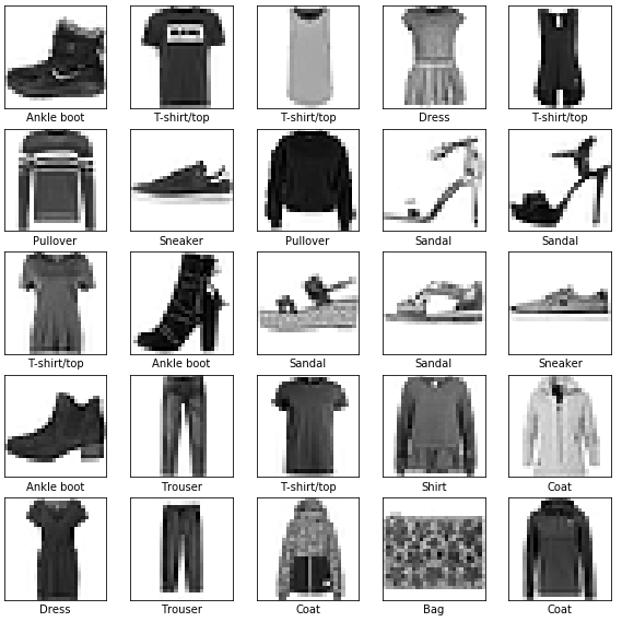
为了验证数据的格式是否正确,以及是否准备好构建和训练网络,让我们显示训练集中的前25张图像,并在每个图像下方显示类名称。
1
2
3
4
5
6
7
8
9
|
plt.figure(figsize=(10,10))
for i in range(25):
    plt.subplot(5,5,i+1)
    plt.xticks([])
    plt.yticks([])
    plt.grid(False)
    plt.imshow(train_images[i], cmap=plt.cm.binary)
    plt.xlabel(class_names[train_labels[i]])
plt.show()
|
建立模型
建立神经网络需要配置模型的各层,然后编译模型。
设置图层
神经网络的基本构建模块是层。层从输入到它们的数据中提取特征。希望这些特征对于当前的问题有意义。
深度学习的大部分内容是将简单的层链接在一起。大多数层(例如tf.keras.layers.Dense)都有在训练期间学习的参数。
1
2
3
4
5
|
model = keras.Sequential([
    keras.layers.Flatten(input_shape=(28, 28)),
    keras.layers.Dense(128, activation='relu'),
    keras.layers.Dense(10, activation='softmax')
])
|
网络的第一层tf.keras.layers.Flatten将图像的格式从二维数组(2828像素)转换为一维数组(2828=784像素)。可以将这一层看作是图像中的一行行像素并将它们排列起来。该层没有要学习的参数,它只是重新格式化数据。
像素展平后,网络由两个tf.keras.layers.Dense层组成。这些是紧密连接或完全连接的神经层。第一个密集层有128个节点(或神经元)。第二层(也是最后一层)是有10个节点的softmax层,该层返回一个含有10个概率值的数组,其总和为1。每个节点都包含一个分数,该分数表示当前图像属于哪个类别的概率。
编译模型
在模型准备训练好之前,还需要进行一些设置。这些是在模型的编译步骤中添加的:
- 损失函数:衡量训练期间模型的准确性。你希望最小化此函数,以便将模型“引导”到正确的方向上。
- 优化器:这是基于模型看到的数据及其损失函数来更新模型的方式。
- 指标:用于监控训练和测试步骤。下面的例子使用准确性,即正确分类的图像比例。
1
2
3
|
model.compile(optimizer='adam',
              loss='sparse_categorical_crossentropy',
              metrics=['accuracy'])
|
训练模型
训练神经网络模型需要执行以下步骤:
- 将训练数据输入模型。在本例中,训练数据为
train_images和train_labels数组。
- 与模型学习关联的图像和标签。
- 要求模型对测试集(在本例中为
test_images数组)做出预测。验证预测是否与test_labels数组中的标签匹配。
调用model.fit方法开始训练,之所以这么称呼是因为该方法使模型“适合”训练数据:
 1
 2
 3
 4
 5
 6
 7
 8
 9
10
11
12
13
14
15
16
17
18
19
20
21
22
23
24
25
|
model.fit(train_images, train_labels, epochs=10)

Train on 60000 samples
Epoch 1/10
60000/60000 [==============================] - 5s 85us/sample - loss: 0.4978 - accuracy: 0.8245
Epoch 2/10
60000/60000 [==============================] - 4s 69us/sample - loss: 0.3798 - accuracy: 0.8624
Epoch 3/10
60000/60000 [==============================] - 4s 62us/sample - loss: 0.3411 - accuracy: 0.8762
Epoch 4/10
60000/60000 [==============================] - 4s 61us/sample - loss: 0.3164 - accuracy: 0.8838
Epoch 5/10
60000/60000 [==============================] - 4s 61us/sample - loss: 0.2956 - accuracy: 0.8902
Epoch 6/10
60000/60000 [==============================] - 4s 64us/sample - loss: 0.2815 - accuracy: 0.8955
Epoch 7/10
60000/60000 [==============================] - 4s 65us/sample - loss: 0.2691 - accuracy: 0.9009
Epoch 8/10
60000/60000 [==============================] - 4s 62us/sample - loss: 0.2579 - accuracy: 0.9029
Epoch 9/10
60000/60000 [==============================] - 4s 63us/sample - loss: 0.2485 - accuracy: 0.9062
Epoch 10/10
60000/60000 [==============================] - 4s 60us/sample - loss: 0.2388 - accuracy: 0.9100

<tensorflow.python.keras.callbacks.History at 0x7fefe642a860>
|
模型训练时,会显示损失和准确度指标。该模型在训练数据上达到0.88(或88%)的准确度。
评估准确性
接下来,比较下模型在测试数据集上的表现:
1
2
3
4
5
|
test_loss, test_acc = model.evaluate(test_images,  test_labels, verbose=2)
print('\nTest accuracy:', test_acc)

10000/1 - 1s - loss: 0.2934 - accuracy: 0.8830
Test accuracy: 0.883
|
结果表明,测试数据集的准确性略低于训练数据集的准确性。训练准确性和测试准确性之间的差距代表过拟合。过拟合是指机器学习模型在新的、看不见的输入上的表现比训练数据上的表现差的情况。
作出预测
通过训练模型,你可以使用它来预测某些图像。
1
|
predictions = model.predict(test_images)
|
这里,模型已经预测了测试集中每个图像的标签。让我们看一下第一个:
1
2
3
4
5
|
predictions[0]

array([1.06123218e-06, 8.76374884e-09, 4.13958730e-07, 9.93547733e-09,
       2.39135318e-07, 2.61428091e-03, 2.91701099e-07, 6.94991834e-03,
       1.02351805e-07, 9.90433693e-01], dtype=float32)
|
预测是由10个数字组成的数组。它们代表模型对应于10种不同服装中的每一种的“把握”。你可以看到哪个标签的置信度最高:
1
2
|
np.argmax(predictions[0])
9
|
因此,模型最有把握的图像是ankle boot或class_names[9]。检查测试标签表明此分类是正确的:
以图形方式查看完整的10个类的预测。
1
2
3
4
5
6
7
8
9
10
11
12
13
14
15
16
17
18
19
20
21
22
23
24
25
26
27
28
29
30
|
def plot_image(i, predictions_array, true_label, img):
  predictions_array, true_label, img = predictions_array, true_label[i], img[i]
  plt.grid(False)
  plt.xticks([])
  plt.yticks([])

  plt.imshow(img, cmap=plt.cm.binary)

  predicted_label = np.argmax(predictions_array)
  if predicted_label == true_label:
    color = 'blue'
  else:
    color = 'red'

  plt.xlabel("{} {:2.0f}% ({})".format(class_names[predicted_label],
                                100*np.max(predictions_array),
                                class_names[true_label]),
                                color=color)

def plot_value_array(i, predictions_array, true_label):
  predictions_array, true_label = predictions_array, true_label[i]
  plt.grid(False)
  plt.xticks(range(10))
  plt.yticks([])
  thisplot = plt.bar(range(10), predictions_array, color="#777777")
  plt.ylim([0, 1])
  predicted_label = np.argmax(predictions_array)

  thisplot[predicted_label].set_color('red')
  thisplot[true_label].set_color('blue')
|
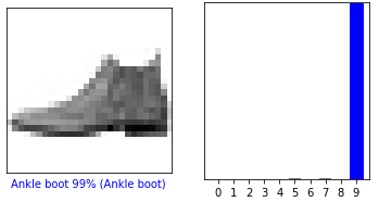
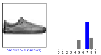
让我们看一下第0张图片的预测和预测数组。正确的预测标签为蓝色,错误的预测标签为红色。数字给出了预测标签的百分比。
1
2
3
4
5
6
7
|
i = 0
plt.figure(figsize=(6,3))
plt.subplot(1,2,1)
plot_image(i, predictions[i], test_labels, test_images)
plt.subplot(1,2,2)
plot_value_array(i, predictions[i],  test_labels)
plt.show()
|
1
2
3
4
5
6
7
|
i = 12
plt.figure(figsize=(6,3))
plt.subplot(1,2,1)
plot_image(i, predictions[i], test_labels, test_images)
plt.subplot(1,2,2)
plot_value_array(i, predictions[i],  test_labels)
plt.show()
|
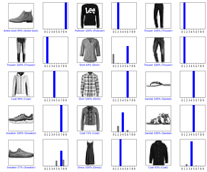
让我们用它们的预测来绘制几个图像。请注意,即使非常有把握,该模型也可能是错误的。
 1
 2
 3
 4
 5
 6
 7
 8
 9
10
11
12
13
|
# Plot the first X test images, their predicted labels, and the true labels.
# Color correct predictions in blue and incorrect predictions in red.
num_rows = 5
num_cols = 3
num_images = num_rows*num_cols
plt.figure(figsize=(2*2*num_cols, 2*num_rows))
for i in range(num_images):
  plt.subplot(num_rows, 2*num_cols, 2*i+1)
  plot_image(i, predictions[i], test_labels, test_images)
  plt.subplot(num_rows, 2*num_cols, 2*i+2)
  plot_value_array(i, predictions[i], test_labels)
plt.tight_layout()
plt.show()
|
最后,使用经过训练的模型对单个图像进行预测。
1
2
3
4
5
|
# Grab an image from the test dataset.
img = test_images[1]
print(img.shape)

(28, 28)
|
tf.keras对模型进行了优化,可以同时对一批或一组示例进行预测。因此,即使你使用的是单个图像,也需要将其添加到列表中:
1
2
3
4
5
|
# Add the image to a batch where it's the only member.
img = (np.expand_dims(img,0))
print(img.shape)

(1, 28, 28)
|
现在,为该图像预测正确的标签:
1
2
3
4
5
6
7
8
|
predictions_single = model.predict(img)
print(predictions_single)

[[1.4175281e-04 8.5218921e-14 9.9798274e-01 1.7262291e-11 1.3707496e-03
  1.4081123e-14 5.0472573e-04 6.2876434e-17 3.6248435e-09 1.8519042e-13]]]

plot_value_array(1, predictions_single[0], test_labels)
_ = plt.xticks(range(10), class_names, rotation=45)
|
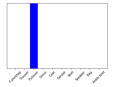
model.predict返回一系列的列表,每一个列对应于批量数据中的每个图像。在批量数据中获取我们(唯一)图像的预测:
1
2
|
np.argmax(predictions_single[0])
2
|
模型按预期预测了一个标签。